Harness the Power of Regression with Python: A Beginner's Guide

 

Introduction

A regression is a statistical technique that helps us analyze and understand the relationship between a dependent variable and one or more independent variables. There are many types of regression the most common models are; Linear regression Polynomial regression and Logistic regression.

In this article, I would like to discuss linear regression including simple linear regression and multiple linear regression, and how to implement this algorithm using Python and scikit-learn (a machine learning library for Python).

Linear Regression

Linear regression is a supervised learning that uses and shows the relationship between the data points to draw a straight line through all of them. This line can be used to predict future values.

Simple Linear Regression

This types of regression uses a single feature i.e. independent variable to determine the dependent variable.

let’s use scikit-learn to implement simple Linear Regression and create a model, train it, test it and use the model.

Importing Needed packages & Downloading Data

In this example, I will use fuelconsumption dataset, which contains model-specific fuel consumption ratings and estimated carbon dioxide emissions for new light-duty vehicles for retail sale in Canada.

import matplotlib.pyplot as plt
import pandas as pd
import pylab as pl
import numpy as np

%matplotlib inline

df = pd.read_csv("FuelConsumptionCo2.csv")

# take a look at the dataset
df.head()

As you can see this contain a lot of features, so let’s select one i.e ENGINE SIZE as the independent variable and CO2 EMISSION as the dependent variable.

cdf = df[['ENGINESIZE','CO2EMISSIONS']]
cdf.head()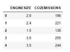

let’s plot each of this features against the Emission, to see how linear their relationship is

plt.scatter(cdf.ENGINESIZE, cdf.CO2EMISSIONS,  color='blue')
plt.xlabel("Engine size")
plt.ylabel("Emission")
plt.show()

Creating train/test dataset and Modeling

from sklearn.model_selection import train_test_split
from sklearn import linear_model


X = np.asanyarray(df[["ENGINESIZE"]])
y = np.asanyarray(df[["CO2EMISSIONS"]])

X_train,X_test,y_train,y_test = train_test_split(X,y,test_size=0.2)

regr = linear_model.LinearRegression()
regr.fit(X_train, y_train)

# The coefficients
print ('Coefficients: ', regr.coef_)
print ('Intercept: ',regr.intercept_)

output:
  Coefficients:  [[39.86432526]]
  Intercept:  [122.8486243]

Plot output: We can plot the fit line over the data.

plt.scatter(X_train, y_train,  color='blue')
plt.plot(X_train, regr.coef_[0][0]*X_train + regr.intercept_[0], '-r')
plt.xlabel("Engine size")
plt.ylabel("Emission")

Evaluation

from sklearn.metrics import r2_score

y_pred = regr.predict(X_test)

print("Mean absolute error: %.2f" % np.mean(np.absolute(y_pred - y_test)))
print("Residual sum of squares (MSE): %.2f" % np.mean((y_pred - y_test) ** 2))
print("R2-score: %.2f" % r2_score(y_test , y_pred) )

output:
Mean absolute error: 22.78
Residual sum of squares (MSE): 908.26
R2-score: 0.78

As you can see the model accuracy is around 80%