Exploring Clustering Algorithms: How to Master the Art of Data Grouping with Python

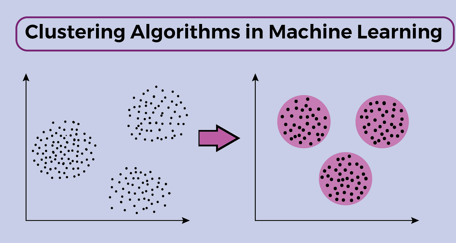
What is Clustering?

Clustering is a type of Unsupervised Learning. it refers to a set of techniques for finding subgroups or clusters (collections of data based on similarity) in a dataset.

Clustering Algorithms

Clustering techniques are used for investigating data, identifying anomalies, locating outliers, or seeing patterns in the data. There different types of clustering Algorithms in machine learning,these include;

• K-Means clustering
• Mini batch K-Means clustering algorithm
• Hierarchical Agglomerative clustering.
• density-based clustering algorithm (DBSCAN)

In this blog post, I would like to explore K-Means clustering Algorithms, how it works, and how to implement it with Python and Scikit-learn.

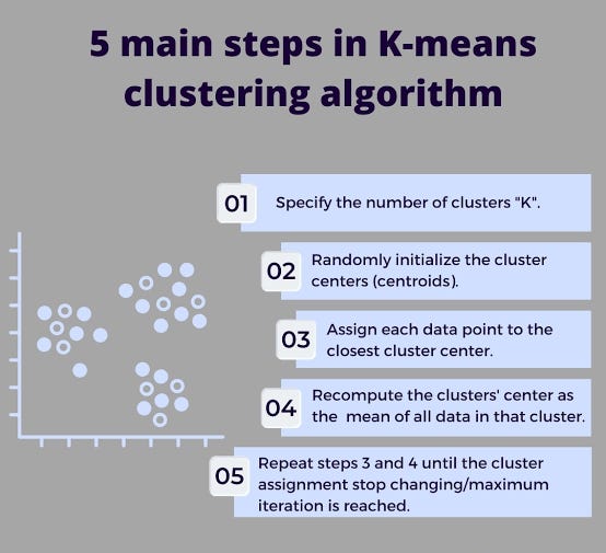
K-Means Clustering Algorithms
In K-Means, Centroids are calculated via the K-means clustering algorithm, which then iterates until the best centroid is discovered.

How K-Means Clustering Algorithms Work?

K-Means steps

Implementation

Import libraries

import random 
import numpy as np 
import matplotlib.pyplot as plt 
from sklearn.cluster import KMeans 
from sklearn.datasets import make_blobs 
%matplotlib inline

Create Dataset

Let’s create our own dataset . First we need to set a random seed. Use numpy’s random.seed() function, where the seed will be set to 0. Next we will be making random clusters of points by using the make_blobs class.

np.random.seed(0)

X, y = make_blobs(n_samples=5000, centers=[[4,4], [-2, -1], [2, -3], [1, 1]], cluster_std=0.9)

# Display the scatter plot of the randomly generated data.
plt.scatter(X[:, 0], X[:, 1], marker='.')

Setting up K-Means

Now that we have our random data, let’s set up our K-Means Clustering.Then fit the KMeans model with the feature matrix we created above.

k_means = KMeans(init = "k-means++", n_clusters = 4, n_init = 12)

k_means.fit(X)

Now let’s grab the labels for each point in the model using KMeans’ .labels_ attribute and save it as k_means_labels. Also we get the coordinates of the cluster centers using KMeans’ .cluster_centers_ and save it as k_means_cluster_centers

k_means_labels = k_means.labels_
k_means_labels

output:
  array([1, 0, 0, ..., 1, 2, 1])

k_means_cluster_centers = k_means.cluster_centers_
k_means_cluster_centers

output:
  array([[-2.02895818, -0.97875837],
       [ 2.05176574, -3.00324819],
       [ 4.0006194 ,  3.99431306],
       [ 1.0004603 ,  1.03344555]])

Creating the Visual Plot

So now that we have the random data generated and the KMeans model initialized, let’s plot them and see what it looks like!

# Initialize the plot with the specified dimensions.
fig = plt.figure(figsize=(6, 4))

# Colors uses a color map, which will produce an array of colors based on
# the number of labels there are. We use set(k_means_labels) to get the
# unique labels.
colors = plt.cm.Spectral(np.linspace(0, 1, len(set(k_means_labels))))

# Create a plot
ax = fig.add_subplot(1, 1, 1)

# For loop that plots the data points and centroids.
# k will range from 0-3, which will match the possible clusters that each
# data point is in.
for k, col in zip(range(len([[4,4], [-2, -1], [2, -3], [1, 1]])), colors):

    # Create a list of all data points, where the data points that are 
    # in the cluster (ex. cluster 0) are labeled as true, else they are
    # labeled as false.
    my_members = (k_means_labels == k)
    
    # Define the centroid, or cluster center.
    cluster_center = k_means_cluster_centers[k]
    
    # Plots the datapoints with color col.
    ax.plot(X[my_members, 0], X[my_members, 1], 'w',markerfacecolor=col, marker='.')
    
    # Plots the centroids with specified color, but with a darker outline
    ax.plot(cluster_center[0], cluster_center[1], 'o', markerfacecolor=col,  markeredgecolor='k', markersize=6)

# Title of the plot
ax.set_title('KMeans')

# Remove x-axis ticks
ax.set_xticks(())

# Remove y-axis ticks
ax.set_yticks(())

# Show the plot
plt.show()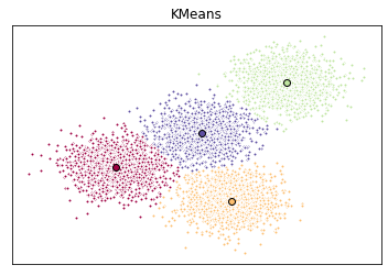

Conclusion

K-means is one of the simplest models amongst the other clustering algorithm, Despite its simplicity, the K-means is vastly used for clustering in many data science applications, it is especially useful if you need to quickly discover insights from unlabeled data.